Probability of Default and Implied Rating Estimation for Corporate Borrowers

Introduction

Internal credit classification processes used by asset managers may differ somewhat from ratings assignment procedures adopted by major nationally recognized statistical rating organizations (NRSROs), such as Moody’s, Standard & Poor’s (S&P), Fitch, etc., in terms of categorization, focus, periodicity, timeliness, and other factors. Nevertheless, the two underlying frameworks also have a number of similarities; for example, they both use qualitative, expert-based assessments of credit quality for issuers, they consider and analyze the same data, and the analytical processes can also be similar.

A qualitative, expert-based approach requires significant credit experience, in-depth understanding of sectoral nuances and repetition over time. In other words, judgment-based schemes need long-lasting experience and evidence that is based on a long window of time covering different market conditions. Thus, while they provide very thorough credit analyses performed by experts, qualitative credit rating processes take time to develop and may have limitations in terms of upwards scalability, timely monitoring of all market signals, and consistency across time and sectors.

To address the potential limitations and enhance the capabilities of the credit assessment process in terms of coverage, consistency and timeliness, many financial institutions have introduced quantitative credit assessment monitoring into their processes. Empowering credit analysts with advanced quantitative credit analysis capabilities helps the experts in terms of timely and more efficient monitoring and expanding the breadth of the credit portfolio names they track.

In this spirit, Western Asset introduced the first version of its Credit Default Model (WISER-CDM) that was integrated into its proprietary risk management system, WISER,¹ in 2019. More recently, Western Asset has reviewed and recalibrated the model, and it is now available for use for risk management, portfolio management and client solutions purposes.

Currently, the WISER-CDM covers publicly traded issuers in developed countries (G7, to be specific), issuers in emerging market (EM) countries, as well as issuers that are not traded (i.e., private) in the corporate credit universe. In addition, the model also provides outputs for municipalities and sovereigns.

In particular, the exact model output is an estimated one-year probability of default (PD) for each entity, along with a PD-implied rating for each issuer. The information is produced and accessible on a daily basis. In addition to being available on a stand-alone basis, the estimated PDs are integrated with the risk simulations in the WISER system so that assessed portfolio-level risk levels also take into account issuer defaults in certain future scenarios of the world.

In this paper, we present an overview of the model and provide some case studies. In particular, we provide a detailed discussion on the data, model structure and model testing, followed by numerical use cases demonstrating the capabilities of the WISER-CDM.

Modeling Framework and Data

The corporate universe for credit analysis can be divided into two segments functionally:

1. Publicly traded credits
2. Private issuers/loans

This segmentation is important, as it affects the modeling choices and framework for our default predictions and credit classification analysis. For the traded-credit universe, we have daily equity market data along with financial statement data available, whereas the private universe only has only the latter available. Accordingly, our modeling framework rests on a hybrid solution with two components:

1. A structural model (à la Merton)
2. A statistical model (reduced form)

Model Component 1: Merton Structural Model
The Merton model, which was proposed by economist Robert C. Merton in 1974, has become one of the pillars for assessing credit risk and assessing a company’s ability to meet financial obligations. The Merton model estimates the structural credit risk of a company by modeling its equity as a call option on its assets. According to this framework, default will occur when the asset value of a company falls below its liabilities (Appendix 1).

Key Assumptions/Logic of Model Component 1:

• The model evaluates the likelihood that the value of a company’s assets will be sufficient to cover its debt obligations (''default point'').
• It assumes that firm value follows a geometric Brownian motion process (akin to a ''random walk'') over time.
• It treats the company’s equity as a call option, with the strike price as the company’s debt.
• In this framework, the difference between expected value of assets and liabilities is expressed in standard deviation units (''distance to default''), which in turn is subsequently translated into a probability that assets fall below liabilities, i.e., the estimated PD.
• Accordingly, default occurs when assets reach a sufficiently low level compared to liabilities.

Exhibit 1: The Merton Structural Model

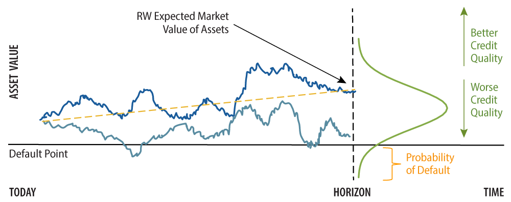
The calculated Distance to Default measure is empirically mapped into physical default rates to assess each issuer’s PD, where there is a separate calibration for financial and non-financial firms to account for differences between the liability structure of two types of companies.

Model Component 2: Statistical ''FinScore'' Model
To (a) be able to provide a credit assessment on credits in the non-traded universe, and (b) for credits in the public universe to complement the Merton model that uses equity market signals in inferring default probability we also developed a model that utilizes financial statement data (the ''FinScore'' Model).

The FinScore Model can conceptually be thought of as a further refinement of Altman’s Z-Score² Model that was developed using financial statement variables to rank credits (to identify whether they are in the ''distress zone'' or not. In our model, rather than a discrete categorization we employ statistical analyses to assert an explicit probability of default for each credit over a one-year timeframe.

Data
The default data period used in the estimations spans the timeframe between October 2003 and December 2023—except the onset of the COVID-19 shock. The source of all the financial statement data throughout the entire estimation is S&P Capital IQ. Data fields are scrubbed to avoid false NAs and zeros. Outliers are removed. After the cleaning process, the data is transformed in order to standardize it and put it on similar scale. In our estimation we use 20 years’ worth of financial statement data points covering 38,954 unique firms.

Variable Selection
As anyone who has experience in credit markets knows, credit analysts’ favorite ratio lists may vary depending on the individual sectors, particular state of the economy in the business cycle, accounting standards, etc. Typically, credit analysts’ favorite ratios can be fairly complicated to account for complexities in the sector they are focusing on, and these complexities may or may not translate well to other industries, potentially causing consistency issues. Moreover, ratios that require a number of specific accounting items may also significantly impact the coverage universe for the analysis.

Thus, in addressing variable selection our philosophy was: (a) to be prudent in the number of variables in the model, (b) select ratios from a wide range of potential risk categories (rather than picking several from the same category), and finally, (c) to select financial ratios that are well understood and widely available, transparent and, when combined together, to be highly predictive for out-of-sample prediction purposes.

To avoid an ''overfitting'' of the model, we selected a limited number of financial ratios that yield a powerful model. During our selection process, we used statistical tests as well as prior modeling experience to determine which variables to include and exclude from the model. Our list of financial statement (FS) ratios falls under one of the following broad-risk factors of financial performance:

• Profitability (return on assets (ROA))
• Leverage (debt/assets: total debt over assets)
• Debt coverage (EBITDA/interest expense)
• Liquidity (cash/assets)
• Activity (retained earnings over current liabilities (RE/CL))
• Size (total assets)

Estimation and Output
While each of these ratios relates to varying degrees of credit risk, we observe a nonlinear relationship between many of these ratios and a firm’s estimated PD. Furthermore, we also acknowledge that extreme values and scaling inconsistencies may lead to spurious results in econometric modeling. Thus, we transformed the FS variables and used their transformed representations in our logistical estimation function. The estimation equation has binary variables (default/no default) regressed on the transformed FS ratios on the right-hand side, where the regression results are checked by sector and rating for calibration.

Based on empirical experience we have observed that blending the Merton Model with the FS Model delivers superior results in terms of credit signaling accuracy; in which the hybrid signals are informative but less noisy. To attain consistency among sectors and jurisdiction, and for prudency in this version of the model, we have opted for a combination algorithm (rather than allowing for nuances among individual sector and/or jurisdictions). Thus, the final output of the WISER-CDM is a hybrid estimated one-year probability of default for all covered issuers globally as well as for private issuers for which we have financial statement data.

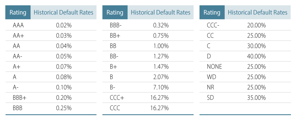
The pros and cons of credit agency ratings are well known in the industry and academia. That said, the fact remains that NRSRO-based ratings are a credit assessment communication tool commonly used by market participants, regulators and clients alike. Therefore, to facilitate better communication and an alternative communication tool, the model also provides PD-implied ratings—utilizing a mapping from estimated PDs to agency ratings, using a stylized table based on default-rate experience by major agency ratings such as Moody’s (Exhibit 2).

Exhibit 2: Historical Default Rates by Rating Bucket

Model Validation
The estimated PDs are validated rigorously for model power and goodness of fit. When the dependent variable Y is a binary variable (i.e., for binary classification or prediction of binary outcomes including binary choice models in econometrics), several statistics can be used to quantify the quality of such models: the area under the receiver operating characteristic (ROC) curve, Kendall's tau (Tau-a), Somers’ D, etc.

Somers’ D is probably the most widely used of the available ordinal association statistics. Identical to the Gini coefficient, Somers’ D is related to the area under the receiver operating characteristic curve, which is labeled as ''Area Under ROC Curve'' – or ''AUC'' for short, wherein:

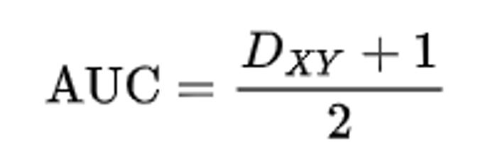
Note that a ''random'' outcome would reveal a Somers’ D score of 0 (whereas for AUC it is 50%) and a perfect model would imply 100%. Thus, in order to test the model’s predictive power, we compute Somers’ D, where the closer the statistics are to unity the more predictive the underlying model is.

Accordingly, the Somers’ D statistics for the estimated model is calculated to be 71.6%. Thus, the model is assessed to be notably powerful in predicting defaults one year ahead and identifying weaker credits.

In addition, we also wanted to examine if movements in estimated PD-implied ratings can be utilized in forecasting future agency ratings. To test this question, we have created a ''confusion matrix'' correlating movements in S&P ratings with movements in PD-implied ratings in the period 12 months ahead of time (i.e., it correlates moves in S&P ratings one year before a CDM move). In principle, a confusion matrix (Exhibit 3) divides the total outcomes in potential buckets, such as ''true positives'' (TP), ''true negatives'' (TN), ''false positives'' (FP) and ''false negatives'' (FN).

We are particularly interested in the ''precision'' of the model; the precision of a model prediction is defined as precision = TP / (TP + FP). According to the confusion matrix data, the precision of the model is calculated to be 75%, where the ratio of (TP + TN) / (TP + FN + FP + TN) turns out to be 41%.

Exhibit 3: Confusion Matrix

Exhibit 4: Confusion Matrix—WISER CDM-Implied Rating vs. S&P Rating Moves

WISER Integration
We include the estimated issuer one-year PDs in our daily WISER simulation runs to assess the magnitude of default risk that portfolios may contain—in addition to the systematic and idiosyncratic factor loadings on credits—and we aggregate these at the portfolio level. WISER risk metrics, such as ex-ante volatility (and tracking error), value at risk (VaR) and expected shortfall (ES) are all inclusive of credit default risk.

On systematic factors, WISER first decomposes each financial instrument in the portfolio and benchmark into a set of risk factor exposures such as yield curves, credit spreads and foreign exchange (FX) rates. The potential future return of each instrument is a function of its exposures to risk factors and changes in risk factors. Once volatilities and correlations between risk factors are estimated, the system then simulates 10,000 possible versions of the economic and financial future (i.e., Monte Carlo simulation) and values portfolios and benchmarks in those simulated future states. In the simulation, some risk factors have significantly fatter tails than implied by the normal distribution assumption. The WISER model uses the Student’s t-distribution assumption to capture fat-tailed behavior observed in most financial time series.

An issuer may experience defaults in some of the simulated states as driven by the estimated PD. The loss from rare but impactful default events can materially change tail-risk behavior of some portfolios, in addition to the non-normal distribution assumption of the systematic factors described earlier.

Examples: WISER-CDM—Case Studies

In this segment we would like to present some practical examples of how WISER PDs and PD-implied ratings may be of use to credit analysts.

The first case pertains to Royal Caribbean Co. (RCL), and the second case study touches on NAIC-related uses of the model output using Rogers Communications (RCI). In the following graphs, the x-axis indicates the time, and the vertical y-axis displays the rating. Finally, we also show some evidence of the predictive power of the model in terms of providing signals for National Association of Insurance Commissioners (NAIC) rating classification changes.

In the following graphs, the time series in blue shows the PD-implied rating and the plot in green shows the S&P rating.

Royal Caribbean Case Study
Accordingly, we observe that RCL was upgraded twice by S&P (green line) since 2023 (moving from single B to BB+). On the same graph, we note that the blue graph moves ahead of rating changes – thus signaling a rating change months ahead of actual rating action by S&P. Thus, we observe that the Implied rating change has some signaling power predicting a forthcoming agency rating adjustment for RCL (in 2023 and 2024).

Exhibit 5: Royal Caribbean, Historical PD-Implied Ratings vs. S&P Ratings

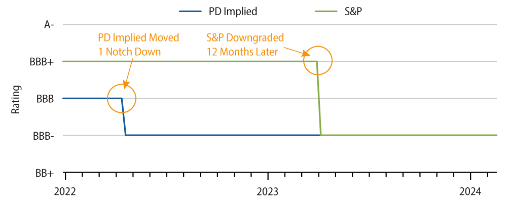
Rogers Communications Case Study
Similarly, Exhibit 6 displays the agency and PD-Implied rating history for Rogers Communications (RCI).

In this example, we note that RCI was downgraded by two notches in 2023 (going from BBB+ to BBB-). We further observe a more conservative rating from Western Asset’s PD than from S&P at the beginning of the period. The subsequent move in the implied rating from our PD came one year ahead of S&P’s move. Further, other NAIC credit rating providers (such as Moody’s, Fitch and DBRS Morningstar) downgraded RCI around the same time as S&P.

Exhibit 6: Rogers Communications, Historical PD-Implied Ratings vs. S&P Ratings

Predicting Changes in NAIC Rating Classifications
Another potential application of the WISER PD-implied ratings can be in the context of NAIC rating classifications. Insurance companies in the US are bound by NAIC rules for calculation of their capital charges. To avoid a cliff in NAIC charges, NAIC adopted a somewhat more granular methodology in ranking credit quality a few years ago. The WISER-CDM model might be helpful to project potential downgrades and security reclassification that could impact capital charges for insurers.

The rule can roughly be summarized as:

• If only one rating is available, use that one.
• If there are two ratings available, use the lower of the two ratings.
• If there are three or more ratings available, use the second lowest, even if the two lowest ratings are the same.

Exhibit 7: NAIC Designation Classification

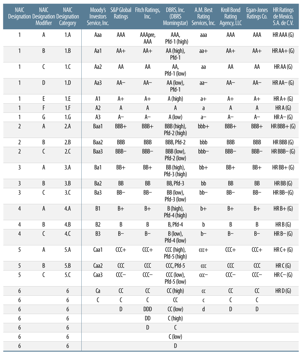
Accordingly, to test if our model can be utilized to forecast changes in NAIC classifications we conducted the following experiment:

Similar to our standardized implied-rating mapping for each credit, for the rated universe with known ratings we mapped the estimated PDs into a ''NAIC Designation Category.'' Accordingly, we repeated the same process for the PD-implied ''NAIC Designation Category'' ratings, where we have correlated the actual NAIC categorization moves with moves in our implied ratings 12 months ahead of time and generated this confusion matrix:

Exhibit 8: Confusion Matrix, NAIC vs. WISER-CDM-Implied Ratings

Following the same notations and formulae we find that the precision of the PD-implied NAIC designations is about 68%. Given the high number of ''no moves'' in NAIC, the ratio of (TP + TN) / (TP + FN + FP + TN) turns out to be somewhat lower, i.e., 38%. Thus, changes in the model can be utilized as a signal for the credit analysis process.

APPENDIX

1: Default Point
Merton defines the Distance to Default (DD) of a firm as:

A common practice of defining ''default point'' is current liabilities + 0.5 * long-term liabilities (which originates from various research and has been implemented in academic literature). Empirical tests suggest that this definition works well for non-financial companies. However, this definition may result in problems for financial firms, mainly due to reporting practices. Hence, for financials, we use a different variation: Long-Term Debt + 0.5 * Total Deposit for US Banks.

2: Equity Value, Asset Value and Volatility in the Merton Model
To compute DD, we first need to estimate the asset value and asset volatility (both are non-observable). As Hull and White (2004) show:

Where E0 is the equity value (at time=0), A0 is the asset value, and:

And, as shown by Jones et al. (1984), because the equity value is a function of the asset value, we can use Itô’s lemma to determine the instantaneous volatility of the equity from the asset volatility:

Where σE is the instantaneous volatility of the company’s equity at time zero. From equation (1). This leads to:

Equations (1) and (2) allow A0 and σA to be obtained from E0, σE, L and T, where L a measure of leverage, i.e., L = D / A.

Thus, to estimate the model, the necessary inputs are equity price, equity volatility, short-term and long-term debt to calculate the default point and the risk-free interest-rate data.

---