ESG and Bond Portfolio Performance

Introduction

While many studies have examined the effect of environmental, social and governance (ESG) quality on portfolio performance, the majority of these analyses have focused on portfolios that consist of public equities. As fixed-income specialists, we set out to address the question from a bondholder perspective. We analyzed approximately 10 years of bond pricing and analytics data from the Bloomberg Barclays US Corporate Bond Index (ticker: LUACTRUU) (also known as the Corporate Bond Index), and issuer-level ESG scores from MSCI ESG Research. The two questions we focused on were:

1. Are higher ESG scores associated with higher future returns in bond markets across sectors?
2. Can one improve on ESG-driven return predictions by employing non-linear machine learning (ML) models?

In this paper, we first introduce the data sets involved in our study; second, we explain how we construct portfolios to examine how ESG affects bond portfolio performance; third, we describe our method to backtest the effect of ESG on bond portfolio performance; finally, we apply ML models to construct our own proprietary return predictions based on ESG subfactors that exhibited a stronger relationship than top-level ESG scores to performance in terms of alpha.

About the Data

We collected and merged data from three distinct sources: 1) bond-level analytics and returns data on the Corporate Bond Index, which is comprised of investment-grade rated fixed-income issuers in the USD-denominated market; 2) MSCI ESG issuer rating scores, which are generated primarily for equity issuers; and 3) the S&P Capital IQ financial database, to facilitate the linkage between issuers in equity and bond markets.

MSCI’s methodology² to determine issuer scores and ratings is somewhat complex and arguably subjective. The MSCI ESG framework includes:

• 37 keys issues and opportunities—a subset of which is applicable to each industry. Each key issue/opportunity score is based on a company’s exposure to, and ability to manage, that particular risk.
• E, S and G “pillar scores” are then calculated based on the key issues/opportunities considered relevant to each issuer’s sector, weighted according to an industry-specific framework. The weighted average of these pillar scores of an issuer is normalized by its industry to determine an issuer’s final industry-adjusted score. This industry-adjusted score is then translated into an ESG letter rating (e.g., AAA, BBB) for each issuer.

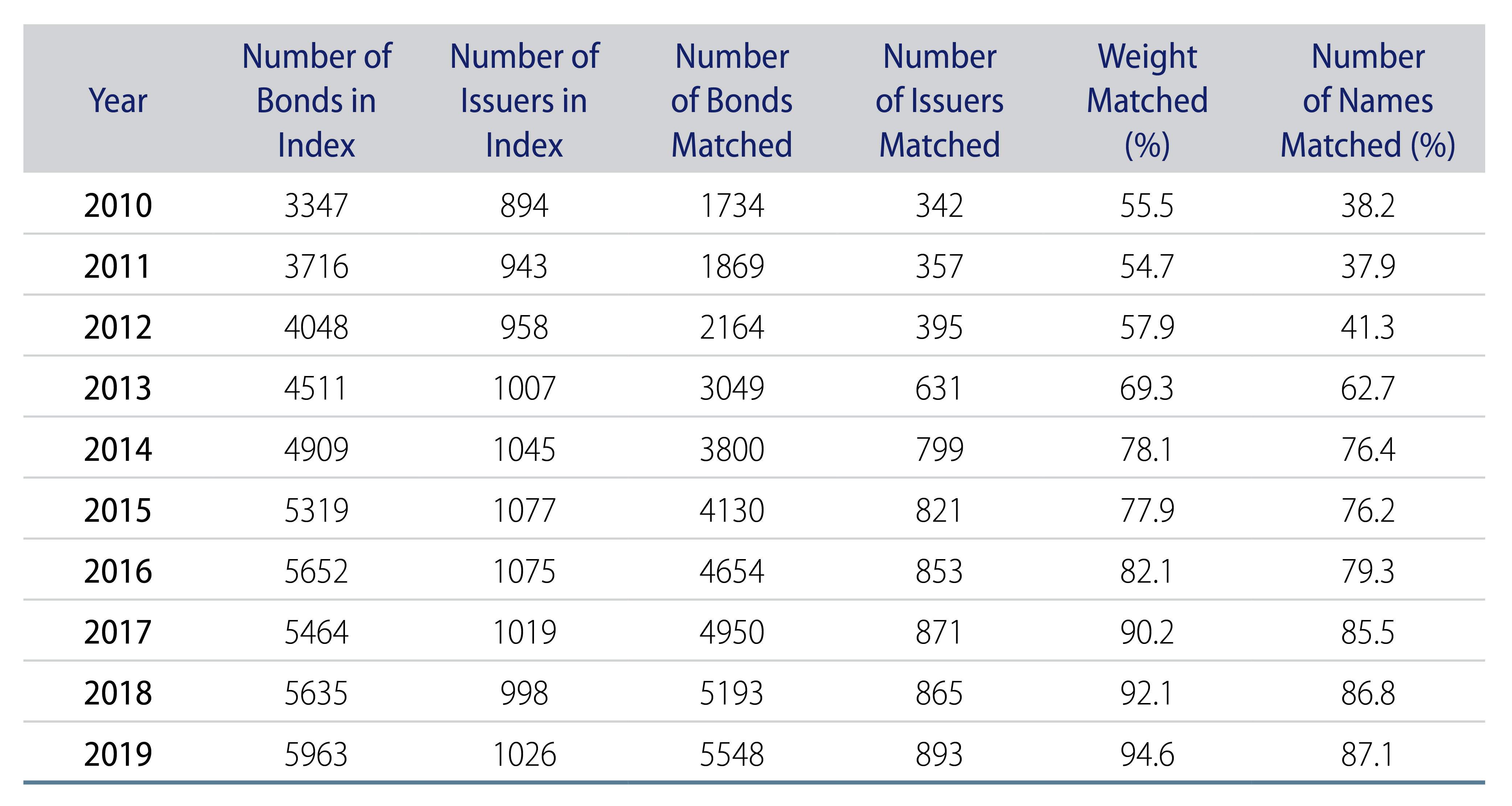
The data set used for this study, which comprises monthly data, covers the period between January 2010 and December 2019. MSCI ESG Research coverage of the Corporate Bond Index is shown in Exhibit 1.

Portfolio Construction

In the corporate credit markets, spread and spread duration are two of the key factors that can affect a bond’s performance. Credit spread is a measure of credit risk in the form of expected compensation over government bonds. Spread duration, on the other hand, measures the sensitivity of a given bond to spread change.

We postulate that ESG characteristics may be associated with differences in other risk attributes. For example, higher-rated issuers tend to have better ESG scores, and there is some relationship between ESG scores and industries as well.

To examine the relationship between ESG factors and financial performance, we need to isolate the ESG-specific factors from the non-ESG-related factors that can impact bond performance. To do so, we constructed a pair of portfolios, one with higher and one with lower MSCI ESG scores. These portfolios were created in several steps:

1. We used market value weights to aggregate bond level data by issuer;
2. We grouped issuers by industry as defined by Global Industry Classification Standard (GICS)³ sectors;
3. We split issuers within each industry into three groups based on their ESG rating score quantile;
4. We assigned the top 1/3 quantile group (with the highest ESG scores) to the “top portfolio” and assigned the bottom 1/3 quantile group (with the lowest ESG scores) to the “bottom portfolio,” removing the middle quantile names from our analysis; and
5. Finally, we assigned equal weight to each issuer in order to control concentration risk in both the top and bottom portfolios.

Exhibit 1: MSCI ESG Research Coverage of the Corporate Bond Index

We recognize that an equally weighted portfolio could create mismatches between spread and spread duration between the top and bottom portfolios. To address the mismatching issue, we used CDX IG and HY 5-year indices as hedging instruments to match both portfolios’ spread and spread duration to the industry sub-index. In our backtesting analysis, which we describe in the next section, we found that the combined hedging instruments accounted for less than 20% of the portfolio volatility in the majority of cases.

To identify any survival bias issues, we looked for bonds that had exited the Corporate Index due to defaults. There were six such bonds that defaulted between January 2010 and December 2019. For these bonds, we assumed a 40% recovery rate to calculate performance. For bonds exiting the index for other reasons, (e.g., below minimum maturity, call option exercise, etc.) we used Bloomberg Barclays index pricing to calculate returns.

Our next step was to backtest the performance of the pair portfolios.

Backtesting ESG Effects

We backtested the portfolios over the period from January 2013 to December 2019. Taking into consideration the necessary amount of data needed to make a statistical inference, we tested two different investment holding horizons: 3 months and 6 months. In order to have more data points to backtest and to align the frequency with MSCI ESG score reporting (which is typically updated on an annual cycle), we rebalanced the pair portfolios at the beginning of each month, kept the portfolio positions constant for the following 3- and 6-month periods, and measured the portfolios’ excess returns. We examined the performance of the top and bottom portfolios to determine ESG effects on bond portfolio performance.

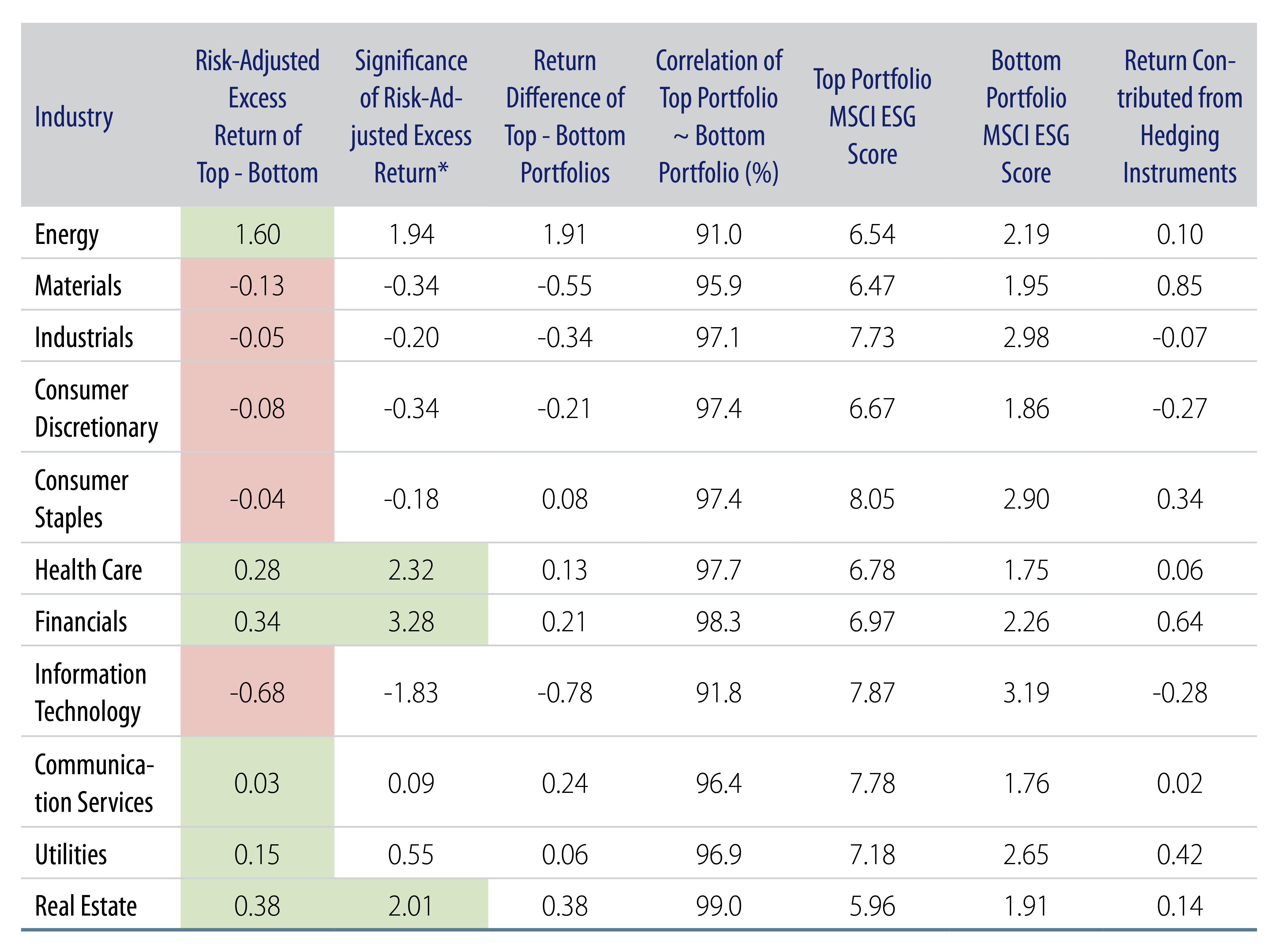
Exhibits 2 and 3 summarize the results based on GICS top-level sectors for the 3- and 6-month holding periods, respectively.

The Results
In Exhibits 2 and 3, the first column, “Risk-Adjusted Excess Return of Top - Bottom,” indicates the difference in annualized returns between the top and bottom portfolios, after adjusting for market risk. To isolate the return impact of volatilities and correlation of top and bottom portfolios, we regressed the 3- and 6-month excess returns of the bottom portfolio to the top portfolio. This first column shows the constant term in the regression, or the alpha in the top portfolio over the bottom portfolio. Positive numbers indicate a positive ESG effect; negative numbers indicate a negative ESG effect.

The second column in Exhibit 2, “Significance of Risk-Adjusted Excess Return,” indicates the statistical significance of the reported excess return in the “Risk-Adjusted Excess Return of Top - Bottom” column. The larger the reported value in absolute terms, the higher the statistical significance of the estimated alpha. Because we rebalanced on a monthly basis (during the investment time period of 3 and 6 months), there are periods of overlap within the backtesting return data. That is, any given set of 3 months of return data has 2 months of overlap and any set of 6 months return data has 5 months of overlap. To address this issue of autocorrelation, we adjusted our T-statistics by using Newey-West estimators.

For the reference and comparison to the first column in Exhibits 2 and 3, the third columns, “Return Difference of Top - Bottom Portfolios,” are the difference of average annualized return of top and bottom portfolios without risk adjustment.

The “Correlation of Top Portfolio ~ Bottom Portfolio” columns show the return correlations between the top and bottom portfolios. Note that the correlations are generally around 90% or more, which indicates that the r squared (which is equal to correlation squared) is high, the beta of the regression is close to 1 and that month-to-month movements are dominated by the overall market moves for the sector. The risk-adjusted return and its significance (first and second columns) show the amount of excess returns after taking out the “beta” of the market return.

“Top Portfolio MSCI ESG Score” and “Bottom Portfolio MSCI ESG Score” are the average MSCI ESG scores in the top and bottom portfolios over each backtesting period.

“Return Contributed from Hedging Instruments” shows the contribution to overall returns from the hedging instruments. The lower the contribution, the lower the importance of the hedging instruments in this analysis.

The results indicate that ESG effects can vary across industries. For example, in the industrials sector, higher ESG scores are associated with negative subsequent returns in a statistically significant way (t-stat is -3.14) for the 3-month holding period, while for the 6-month period the relationship is negative but not statistically significant. Meanwhile, higher ESG scores are associated with positive returns for energy companies in both the 3- and 6-month periods and are around the boundary of statistical significance (t-stat of 2.0). The 3- and 6-month results are generally in line with each other and there are no cases where a statistically significant return becomes statistically significant in the opposite direction when moving from 3 to 6 months. However, there are some sectors with materially different t-stat results that can indicate an increasing or decreasing effect of the ESG rating for longer time periods or (particularly for small differences) statistical noise.

Exhibit 2: Backtesting 3-Month Holding Period Results

Analysis of ESG Subfactors on Returns Using Machine Learning

As explained earlier, MSCI ESG top-level ESG ratings are an aggregation of multiple, more granular subcomponent scores across the three ESG pillars. Some investors may disagree on the materiality of each of the subfactors that feed into the top-level rating and their effect on financial performance. While many studies have re-weighted the subfactors in search of better correlation to financial performance, most of them have used linear models and focused on the public equities market.

Exhibit 3: Backtesting the 6-Month Holding Period Results

ML models provide a potential advantage in examining the relationship between ESG factors and financial performance. They generally excel at capturing non-linear relationships among a large number of variables. In this study, we applied a non-linear ML model to construct different weighting schemes for proprietary ESG return scores (also known as Western Asset ESG return scores), applying the same pair portfolios framework described earlier to evaluate the relationship between Western Asset ESG return scores and subsequent financial performance. This approach was not applied to the real estate sector due to a lack of data history.

For each of these industries, a unique ML model was trained on 37 MSCI subfactors as of the beginning of each year between 2013 and 2019. The models were also calibrated to issuer-level financial performance as of the beginning of the training period. At each monthly rebalancing, we used the beginning-of-year trained models to produce two Western Asset ESG return scores for each issuer across a 3- and 6-month holding period horizon, and constructed a pair of portfolios for each holding horizon, one composed of the top Western Asset ESG return scores quantile, and the other of the bottom Western Asset ESG scores quantile. Thus, the pair of portfolios for the 3-month investment horizon differs from the pair of portfolios for the 6-month time horizon. For example, on 01/01/2013, we trained two models for the industrials subsector for the 3- and 6-month holding period horizons by using ESG granular data from 01//01/2010 to 10/01/2012 and from 01/01/2010 to 07/01/2012, respectively; the subsequent excess returns from the calibration were observed up through 01/01/2013 so that the model training process had no information leakage; then, we applied the trained models at the beginning of each month in 2013.

The results shown in Exhibits 4 and 5 are all out-of-sample results, similar to how we produced the study on MSCI ESG scores before. Comparing the Western Asset ESG return score study with our study of the MSCI ESG scores, the only difference was how we selected the issuers in the top and bottom portfolios. The Western Asset ESG return score study selected names by using our ML model output as rankings for the quantile rather than using the MSCI ESG score as the rankings. As with the MSCI ESG study, we monitored the portfolios’ performance over time by backtesting two different holding periods and rebalancing on a monthly basis. The backtesting period for the MSCI ESG study was January 2013 to December 2019 due to the required amount of training data. Exhibits 4 and 5 show the results for the 3- and 6-month holding periods, respectively.

The Results
A comparison of Exhibits 2 through 5 indicates that the usage of Western Asset ESG return scores results in improved linkage between ESG factors and financial performance versus the usage of aggregate MSCI ESG scores, especially in the 3-month investment horizon. The Western Asset ESG return scores can be used to construct a portfolio that balances return expectations with ESG considerations by showing which subfactors are likely to be additive to returns and which are likely to subtract.

Exhibit 4: Backtesting the 3-Month Holding Period Results

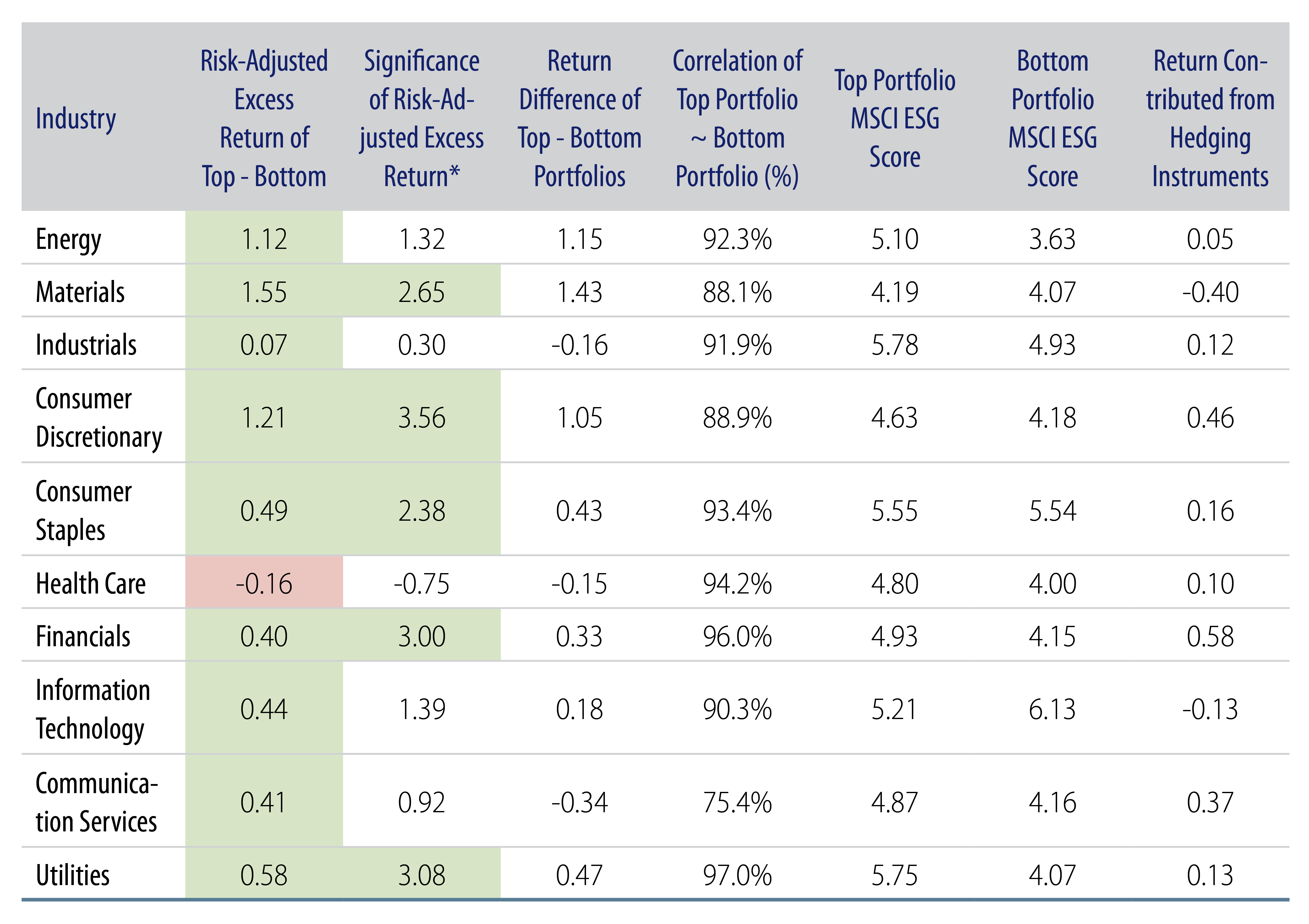
The best ML model for one sector may not be the best model for all sectors. For instance, in the energy sector, the model used in Exhibits 4 and 5 is no better than just using the MSCI aggregate score (Exhibits 2 and 3). The ML model results in a statistical significance (t-stat) of 1.32 versus 2.07 for MSCI score over 3 months. Applying a less complex version of the ML model, with fewer parameters, resulted in a significance of 3.16 for 3-month and 3.01 for 6-month returns. However, the full ML model was generally superior for other sectors.

Exhibit 5: Backtesting the 6-Month Holding Period Results

APPENDIX

Explanatory Note on Model Features
ML models are often non-linear models and explaining “why” a certain result was produced can be difficult. The sensitivity of any one input feature depends on the values of the other input features. In order to interpret ML models in a conventional way, (e.g., sensitivity analysis) we use a linear model to approximate the non-linear ML models that were used. This transformation method is known as the “global surrogate” method and simplifies nonlinearity and/or interactions among the input features. In Exhibit 6, we provide some resulting granular score sensitivities from the model linear proxy. Please note, this approximation does not precisely describe the ML model; it is just one representation of the results.

Exhibit 6: Comparing the ML Models by Industry—Granular Score Sensitivities