

Credit Spread Volatility
Nurture strength of spirit to shield you in sudden misfortune. ~Max Ehrmann, 1927
Executive Summary
- Some credit markets can be characterized as long periods of boredom punctuated by moments of sheer terror. Credit spreads, which capture the higher yields that credit-risky bonds command over non-credit-risky bonds, exemplify this dynamic.
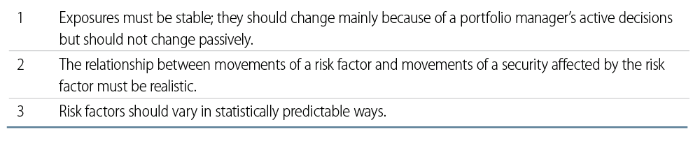
- We define three desiderata that apply to credit spread risk factors and exposures: 1) Exposures must be stable, 2) The relationship between movements of a risk factor and of a security affected by the risk factor must be realistic, and 3) Risk factors vary in statistically predictable ways.
- We analyze the adjusted spread duration (ASD) of securities, which allows for separation of the exposure metric from the risk metric and compare and contrast it with the duration times spread (DTS) metric.
- ASD with time-varying volatility uses an adjustment to spread duration along with a statistical technique to predict time-varying volatility. This combination satisfies all of our desiderata for risk factors and exposures.
Three Desiderata
Successful portfolio construction involves not only the selection of superior securities and investment themes, but also the assessment of the ranges of outcomes of the portfolio’s exposures. The best portfolios carefully balance risk and reward.
An important part of assessing portfolio risk is the identification of risk factors, which are the variables that will affect many or all of the securities in the portfolio. For fixed-income portfolios, some obvious risk factors are the prevailing key rates of interest in the portfolio’s base currency, general levels of credit spreads and foreign exchange rates.
To estimate the range of future returns of a portfolio—either the total return, or the return relative to a benchmark—we need, among other things, to measure or estimate the following information:
- The exposures the portfolio has to its risk factors, and
- The likely ranges of outcomes of those risk factors.
The ranges of outcomes of risk factors can be described statistically. We know for example that over the 10-year period from 2007 to 2016, daily absolute changes in the US Treasury (UST) 10-year rate were less than 13 basis points (bps), 95% of the time. But over the year 2017, the range of UST 10-year daily absolute moves shrank dramatically to less than 7 bps, 95% of the time.
In this note we’ll talk about our approach to estimating credit spread risk. To do this, we need not only identify statistically reliable phenomena, but we also must identify reliable relationships between our portfolio and those phenomena. As such, we target the three desiderata in Exhibit 1.
Desiderata for Risk Factors and Exposures
We’ll discuss each of these, starting with statistical predictability.
Boredom and Terror
As has been said of war, some credit markets can be characterized as long periods of boredom punctuated by moments of sheer terror. Credit spreads, which capture the higher yields that credit-risky bonds command over non-credit-risky bonds, exemplify this dynamic.
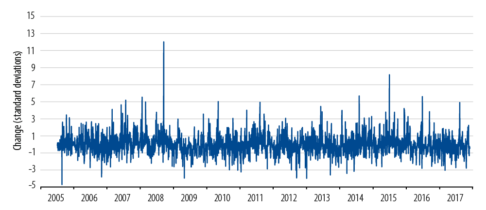
Exhibit 2 shows day-over-day changes in credit spreads for the Bloomberg Barclays U.S. Credit Corporate Index. Each vertical line is a day’s change in spread; for example, the largest upward line in the graph hits 43 bps on the vertical scale. It occurred on September 15, 2008 when the index spread jumped from 327 bps to 370 bps in reaction to the bankruptcy of Lehman Brothers.1
Daily Arithmetic Changes in US Investment-Grade Credit Spreads
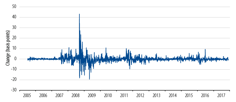
That was sheer terror. The “long periods of boredom” are also apparent here. From November 10, 2011 to January 19, 2016 there wasn’t a single day when spreads changed by more than 6 bps up or down from the previous day.
The credit spread behavior in Exhibit 2 does not satisfy our third desideratum—it is not statistically predictable. One problem is apparent from a visual examination and requires no statistical analysis: there are very large spikes, such as the one on September 15, 2008, that are massively different in magnitude from the usual pattern. The prevalence of such spikes is variously called “fat tails” or “black swans.”2 They are similar to big earthquakes—they don’t happen very often, but when they do they have a huge impact.
Another problem is what financial economists call “volatility clustering.” Again, just by eyeballing Exhibit 2, we can see that daily move amplitude was elevated for about a year before the giant spike on September 15 and continued to be elevated for about a year afterward. This is very much like human emotion: during a period of fear or anxiety, symptoms such as elevated pulse and hyper vigilance persist and possibly lead to panic. But eventually the adrenaline washes out and things cool down.
Standard fixed-income mathematics requires the multiplying of an item’s option-adjusted spread duration3 (OASD) times the item’s credit spread changes (e.g., changes that look like Exhibit 2) to compute the contribution to the item’s rate of return. Although spread duration is a relatively stable quantity, the statistical problems of Exhibit 2 will affect estimation of the range of rates of return through this multiplication.
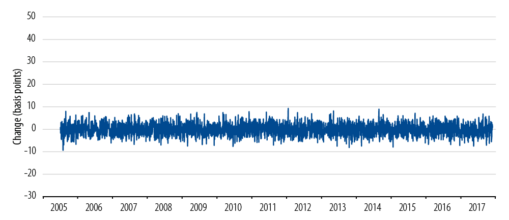
Exhibit 3 shows an ideal world in which the problems of Exhibit 2 have been removed. Exhibit 3 is in simple ways statistically identical to Exhibit 2, with the same average daily move in spreads, and the same volatility of moves in spreads. But we’ve removed the problematic fat tails and volatility clustering.
The world of Exhibit 3 is one in which portfolio managers can anticipate the ranges of outcomes of their decisions quite accurately. This is nice predictable boredom without the terror, which is a good thing when you’re managing portfolios. Is there a way that we can inhabit a world of benign boredom?
Statistically Smooth Simulation of Exhibit 2
The Introduction of Duration Times Spread
In 2005, a group from Lehman Brothers and the Robeco Group5 outlined an approach to dealing with the moments of boredom and terror—the volatility clustering—that credit spreads display.
The authors noted that credit managers looked at exposure measures such as percentage of portfolio holdings and spread duration to assess their credit risk. But the Lehman/Robeco group adduced empirical evidence in favor of duration times spread (DTS) as a better measure.
To illustrate what DTS is and how it works, consider the following sample portfolio consisting of two securities, each comprising half of the portfolio:
- Security A has a spread duration (OASDA) of 3 years and a spread (SA) of 150 bps;
- Security B has a spread duration (OASDB) of 3 years and a spread (SB) of 450 bps.
The percentage holdings—50% for each Security A and Security B—are fairly stable, so they satisfy our first desideratum above.6 But they don’t satisfy the second desideratum: percentage holdings do not provide a realistic picture of the relationship between the security position and the risk of general changes in credit spreads. Longer-duration securities will move more per percent holding than shorter-duration securities, and riskier securities will move more than less risky securities. Using percentage as the exposure measure does not take these effects into account.
Spread duration—or, more accurately, contribution to spread duration—is more widely used by practitioners as an exposure measure. The example portfolio’s spread duration is three years since both component securities have three years’ spread duration. If both Security A’s spread and Security B’s spread widen by 10 bps, the spread duration figure tells us that we expect to lose 30 bps from spread behavior in this portfolio.
But it’s unlikely that A’s spread and B’s spread will widen by the same 10 bps. B is riskier than A, as evidenced by its much higher spread. It is more likely—and is confirmed empirically—that in a general spread widening, B’s spread will move more than A’s spread. For example, suppose some index of general credit spreads is at 150 bps (coincidentally the same as Security A’s spread), and then the index spread widens by 10 bps. Then Security A’s spread is also likely to widen by 10 bps. But Security B will probably widen by something closer to triple that (10 bps times 450 bps divided by 150 bps), or 30 bps.
DTS is a convenient way of doing the accounting for this phenomenon. The DTS of our 50-50 example portfolio is 0.5x3x150+0.5x3x450=900. The index spread widened by 10 bps on a 150 bps base, or 10/150=6.7%. If we multiply 900 times 6.7%, we get an expected 60 bps loss rather than the 30 bps we got from the simple spread duration calculation under the assumption of identical spread changes.
The basic idea of DTS is therefore that the percentage change (6.7% in our example) is the relevant figure to capture spread movement. The arithmetic change (10 bps) is not directly relevant.
Does DTS take us to the ideal world of Exhibit 3? In other words, if we look at percentage changes rather than arithmetic changes, do we get the very predictable pattern of Exhibit 3 rather than the problematic (fat-tailed, volatility-clustered) pattern of Exhibit 2? Exhibit 4 suggests an answer:
Daily Percentage Changes in US Investment-Grade Corporate Credit Spreads
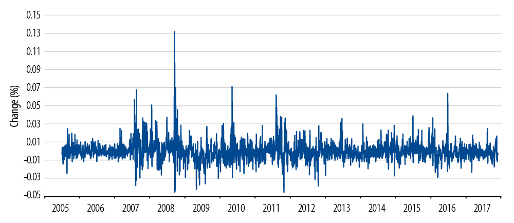
Visually, Exhibit 4 is somewhere between the problems of Exhibit 2 and the regularity of Exhibit 3. There are clearly still fat tails—big movements that differ from the regular pattern far more than anything in Exhibit 3. For example, September 15, 2008 is still clearly visible as an outlier in Exhibit 3—it represents an unusual 13.2% increase in spread. However, it also seems visually clear that there is more regularity in Exhibit 4 than there was in Exhibit 2.7
So from Exhibit 4 and its associated statistics we see that DTS doesn’t quite get us all the way to the nirvana of perfect boredom. But it is a step in the right direction toward Exhibit 1’s third desideratum.
Where Does the Weirdness Go?8
The “trick” in DTS is to confound an exposure measure with a risk measure. In our example above, DTS was 900 at the beginning of the example period. But by the end of the period, DTS was 960—not because the manager increased exposures, but because the market moved.9 DTS removes some unpredictability from the risk factor by transferring that unpredictability to the exposure measure. It improves on delivery of Desiderata 2 and 3 at the expense of desideratum 1.
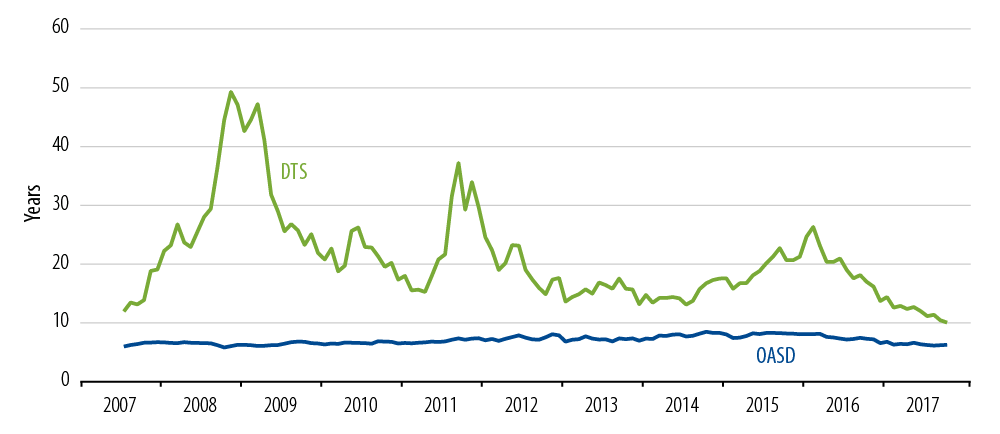
As an example, Exhibit 5 shows the DTS exposure of Western Asset’s Corporate Bond Fund since 2007.
This fund’s option-adjusted spread duration (OASD, blue line) was reasonably smooth over the 10 years shown in Exhibit 5. But the DTS jumped and subsided due to market shocks. The procyclical (lagging indicator) nature of DTS is apparent: DTS would have indicated that exposures were incredibly high just after the worst incidents of spread widening, and that exposures were low during periods of unusually tight spreads.
Thus the increased stability of Exhibit 4 over Exhibit 2 comes at the expense of less stability in the exposure metric, and less clarity about which changes are due to active portfolio manager decisions and which exposures are due to market movements.
Western Asset Corporate Bond Fund DTS and OASD
The standard spread duration approach fails to deliver two of the desiderata, while DTS only fails on one. We are mindful of market strategist M. Loaf’s sage advice: “Two Out of Three Ain’t Bad.”10 Would we be overreaching if we tried to satisfy all three of our desiderata?
Adjusted Spread Duration
There’s another way to do the accounting that gets to the same place as our DTS example without violating desideratum 1. We can look at the adjusted spread duration (ASD) of each security.11 Since Security A has the same spread as the index, we expect changes in Security A to be similar in magnitude to changes in the index. But Security B has a much higher spread, so we adjust its spread duration upward to reflect the likelihood of more intense moves as the index changes.
For our example, we would say ASDA=OASDA=3 years; that is, no adjustment to Security A’s spread duration is needed. But for Security B we would say ASDB=450*OASDB/150=450*3/150=9 years; in other words, we would adjust the spread duration up from 3 years to 9 years. The adjusted spread duration of the 50-50 portfolio is then 0.5x3+.5x9=6 years.
If we apply the portfolio ASD of 6 years to the 10 bps index spread move in our example, we get the same 60 bps loss that we got from DTS. So DTS and ASD attempt to answer a question about what is likely to happen to our portfolio if a general spread level changes, while unadjusted spread duration attempts to answer a question about a not very realistic situation in which every spread in the portfolio changes by the same amount.
ASD is stable and generally not procyclical (desideratum 1). Some adjusted spread durations may change because of market movements, but the fact that the adjustment is made by taking a ratio of credit spreads means that general spread changes will tend not to have too big an effect on overall ASD. Further, ASD’s relationship to risk factor movements is realistic (desideratum 2). Exhibit 6 adds ASD to Exhibit 5, demonstrating ASD’s relative stability.
The ASD is reliably higher than the OASD of the portfolio because the credit spread curve is upward-sloping through virtually the entire period shown, so longer-duration securities get heavier adjustments than shorter-duration securities.
Unfortunately for the return calculation to work properly, we’ve had to revert to arithmetic spread changes (10 bps in the example) as a risk factor. So here, we’ve lost desideratum 3.
Western Asset Corporate Bond Fund DTS, OASD and ASD

Time-Varying Volatility
Fortunately statisticians have studied the nature of time-varying volatility in financial markets. In fact, one of them, Robert Engle, won a Nobel Memorial Prize in Economic Sciences for his work in this area. The model that Engle developed is called ARCH12; this was refined to GARCH13 by Tim Bollerslev and extended by hundreds of researchers over the last three decades.
DTS hard-codes a belief that the immediate current volatility environment (as represented by spread levels) will continue into the future.14 The GARCH-type approach carefully balances three components when making volatility forecasts:
- The current level of volatility;
- The most recent observation—which in our example is a change in credit spreads; and
- A long-term equilibrium level of volatility.
A short-term estimate of volatility will tend to be dominated by the recent environment, while a long-term estimate of volatility will tend to be dominated by the equilibrium level of volatility.
Exhibit 7 shows what happens when we apply GARCH to Exhibit 2.
Time-Varying Volatility Adjustment to Exhibit 2
As with Exhibit 4, Exhibit 7 does not quite bring us to the full predictability of Exhibit 2. There are still surprises. But the statistics16 show that Exhibit 7 mitigates the fat-tail problem even better than Exhibit 4 while virtually eliminating volatility clustering.
With the use of the more powerful time-varying volatility estimation provided by GARCH-type models, we can use adjusted spread duration to realistically assess credit spread risk in portfolios. We can do so in a way that allows portfolio managers to see clearly the effects of their active decisions, avoiding procyclicality. We can separate the activity of describing current risk exposures from the activity of estimating future volatility levels.
Multidimensional Risk
Credit spreads are not monolithic. Short-term credit spreads sometimes part ways with long-term credit spreads; technology spreads don’t always go the same way as financial sector spreads; US credit spreads may diverge from European credit spreads, etc. Thus it’s unrealistic to think that credit spread exposure can be captured with a single number—whether that number is (unadjusted) spread duration, DTS or ASD.
To fully capture credit spread exposures and the associated risks, a multidimensional approach with a full risk model—such as the Western Asset Information System for Estimating Risk (WISER)—is necessary. A full risk model estimates relationships among many types of credit spreads, along with other risk factors.
So when we talk about “the” (unadjusted) spread duration, or “the” DTS, or “the” ASD of a portfolio, we are oversimplifying. It’s like talking about “the” skill of a human being: do we mean skill at playing the piano, or breaking into bank safes, or sailing upwind or managing portfolio risk? We could try to rank a person, say on a scale of 1 to 100, on each of these skills. But it would not make much sense to add these ranks together.
The urge to cram multidimensional effects into a single linear dimension is, however, quite strong. So when we can’t go nonlinear (full-risk system) and we can’t resist the urge to use a single number, we look for a single broad risk factor to use as the denominator of the ASD calculation for all spread-risky securities in a portfolio.
For a broad market US portfolio, we might adjust credit spread durations to give us an idea how that portfolio would react to the risks represented by changes in the Bloomberg Barclays U.S. Credit Corporate Index. For a European high-yield credit portfolio, we might make the adjustment with respect to the Bloomberg Barclays Pan-European High Yield 2% Issuer Constrained Index. This means that the same high-yield security might show a different ASD depending on the benchmark of the portfolio it’s in. So adjusted spread durations are properties of a pair (security, benchmark) and not of the security alone.
Internally at Western Asset, we have assigned reference indices used for the ASD adjustment on a strategy-by-strategy basis. For example, for long duration portfolios a long investment-grade credit index OAS is used for the adjustment. For high-yield portfolios, a high-yield index OAS is used.
Summary
We’d like to have an approach to assessing credit spread risk that satisfies the desiderata in Exhibit 1. This would give us better information as we seek to estimate risk in portfolios.
The standard approach to estimating credit spread risk is to compute spread duration exposures, while using arithmetic changes in general spread levels to represent overall credit spread risk. But a change in general spread levels will not flow through realistically to individual securities using this approach, and the statistical properties of arithmetic changes in spreads are not as steady as we’d like.
The DTS approach improves on some of the failings of the standard approach, but at the expense of creating unstable procyclical exposures with a hardwired view of future volatility.
Using an adjustment to spread duration along with a powerful statistical technique to predict time-varying volatility gets us the best of all worlds, satisfying all the desiderata. The evolution of approaches is shown in Exhibit 8.
Use of Adjustment to Spread Duration With Statistical Technique to Predict Time-Varying Volatility

In fact any combination of quantitative and qualitative assessments can be used to assess likely future risk levels. For example, in the low market volatility environment that prevails at the time of this writing, we believe that portfolios will display unusually low volatility over the short term. But we also believe that over the longer term, there will be a return to a higher volatility environment. The adjusted spread duration method allows us to separate this assessment from the assessment of our exposures.
Three out of three ain’t bad.
Endnotes
- Ironically, the index that captured this behavior was created and computed by Lehman Brothers itself. The fixed-income index business originated by Lehman was taken over by Barclays in 2008 and sold to Bloomberg L.P. in 2016.
- The use of the phrase “Black Swan” to indicate rare but impactful phenomena was popularized by Nicholas Nassim Taleb in his 2007 book The Black Swan: The Impact of the Highly Improbable. The actual statistic that describes tail thickness is kurtosis; fat tails are called leptokurtosis. Virtually all financial time series data are leptokurtic.
- See Appendix for a definition of option-adjusted spread duration.
- Exhibit 2 contains 3,100 daily observations of spread changes. Exhibit 3 was generated by taking 3,100 random numbers drawn from a normal distribution with the same mean and standard deviation as the observations in Exhibit 2.
- Ben Dor, Dynkin, Hyman, Houweling, van Leewun, and Penningo, “A New Measure of Spread Exposure in Credit Portfolios,” Lehman Brothers, June 21, 2005. The group at Lehman was taken over by Barclays and later self-published a follow-up book, “A Decade of Duration Times Spread (DTS),” in 2016.
- Of course percentage holdings do change in buy-and-hold portfolios as mark-to-market prices change, but this effect is relatively slow compared to other effects we will discuss.
- For the statistical reader, the kurtosis of the observations in Exhibit 2 is 50.6, while Exhibit 4’s kurtosis drops to 15.8. The serial correlation of squared observations in Exhibit 2 is 27.6%, while the serial correlation of squared observations in Exhibit 4 is 23.7%.
- Where Does the Weirdness Go? is the title of a 1996 book about quantum mechanics by David Lindley.
- We have actually assumed a rebalancing back to 50-50 weights in our example. In practice there would be an interaction between rate and spread movements that would complicate this calculation.
- Jim Steinman, “Two Out of Three Ain’t Bad,” from Meat Loaf’s Bat Out of Hell, 1977.
- The adjustment leading to the “A” in “ASD” is the proportional spread multiplier defined more precisely in the Appendix. This is in addition to the industry convention of adjusting for optionality in securities, usually denoted “OASD.” ASD is thus both spread-proportion adjusted and option-adjusted.
- ARCH stands for Auto-Regressive Conditional Heteroskedasticity.
- GARCH puts the word “Generalized” in front of ARCH. Tim Bollerslev, “Generalized Autoregressive Conditional Heteroskedasticity,” Journal of Econometrics 31 (1986) 307-327.
- In response to the kinds of problems we have noted, Barclays eventually suggested modifications to DTS. Instead of using “spot” spread, in some cases they use a smoothed (over time) spread. They also recommend restricting the range of spreads over which DTS is used. Our view is that Occam’s Razor applies here: if you have to make a lot of changes to the original idea to get it to work, it’s time to scrap it and start over.
- Exhibit 7 was generated by applying an exponentially weighted moving average (EWMA) variance adjustment to Exhibit 2. This is a simplified form of GARCH.
- Kurtosis was 7.3; serial correlation of squared observations was 0.04.